Video Photometry with Tangra - Algorithms and Acuracy
Using Digital Filters to Improve S/N and Detectability
A new feature in Tangra is the ability to apply a digital filter to the video before processing it. A reason you may want to do this is to improve the signal to noise ratio and make the stars more detectable. Low and high pass filters are often used in modern astronomy for improving the signal to noise ratio for example when detecting stars. The signal of a noisy digital image can frequently be enhanced by suppressing high spatial frequency noise in the image, which in modern CCD stellar observations means suppressing photon and CCD readout noise and can be accomplished by using a small low-pass (LP) filter ([4] Mighell, K., 1999). The same also suppresses noise added during the video rescaling, encoding and compression.Using a Low-Pass Filter
Using a digital filter modifies the raw image which is also done by applying dark and flat fields. However while it is known that applying dark and flat fields improves the signal there is a question of how a digital filter would change the linearity of the intensities in a video. This is what I will try to measure for the LP filter with the next test. Tangra implements its low-pass filter as a non FFT convolution using the following 3x3 kernel: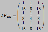
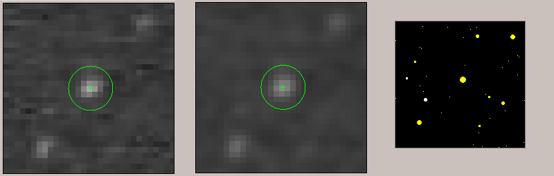
The images on the right show the video frame before and after the LP filter is applied and also show the actual field from the NOMAD catalog. Because the video frame aspect has been changed the distances on the X and Y axis will have different ratio when comparing the video images to the star catalog plot.
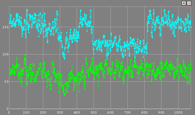
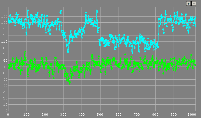
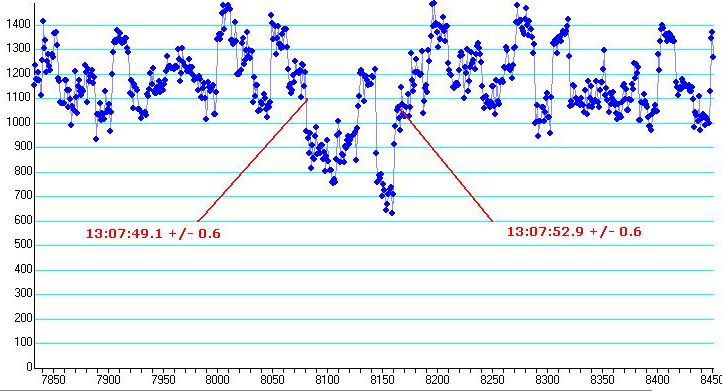
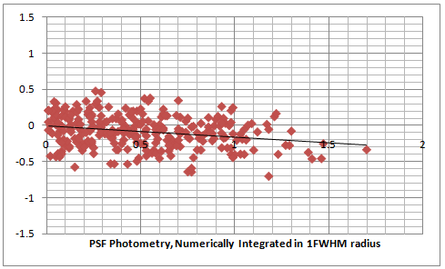
The low-pass filter is nothing more than a very small Gaussian blur. What this means is that objects in the video that have Gaussian distribution such as stars will be enhanced while noise and hot pixels will be suppressed. This is good for getting a better value for the background noise for aperture photometry and is also good for PSF photometry because the real stars will fit better to a Gaussian PSF. The two plots below demonstrate the visible improvement to the S/N in the individual frames when using PSF photometry with an LP filter. A measurement of the occultation of (106) Dione is shown where the left plot is retrieved using PSF photometry with no filter and the right plot is retrieved using PSF photometry with a low-pass filter. The noise is significantly less on the second plot.
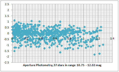
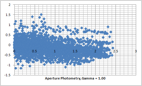
And next we are going to test how an LP filter would affect the photometrtic fit across all stars in the field when used with aperture photometry. I measured a video of M7, which is not used in other measurements so far, and which was recorded with no gamma correction. The two plots below show aperture photometry results without a filter (on the left) and with a low-pass filter (on the right). The raw data can be downloaded here and it also contains a comparison between PSF photometry with and without a low-pass filter.
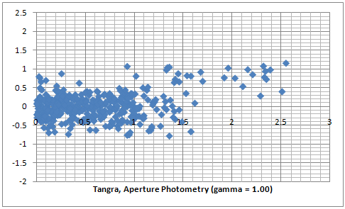
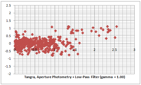
Comparing the plots they look almost exactly the same so we can conclude the effects from an LP filter on the linearity of the magnitudes derived from intensities across the entire image are neglectable.
Using a Low-Pass Difference Filter
A high-pass filter such as the low-pass difference (LPD) filter can be used to better detect fainter stars and has been successfully used with Hubble Space Telescope WF/PC and WFPC2 images for that purpose. Using an LPD filter for asteroid occultations where the target is faint could help to get a more certain light curve and could increase the confidence in detecting or rejecting occultations involving faint targets or short noisy drops. Tangra implements the LPD filter as: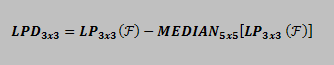 |
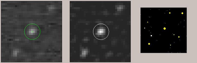 |
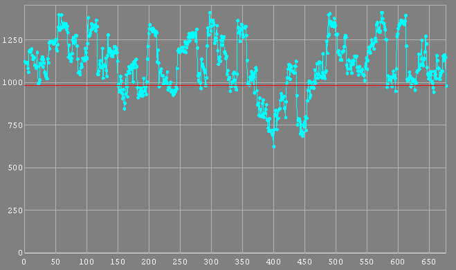
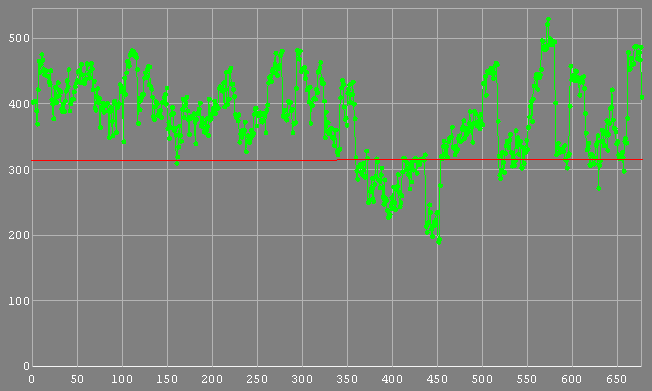
The image on the right shows the video frame before and after applying the LPD filter. The most of the noise has been removed and potential objects have emerged more clearly from the background. In a video if those objects are getting detected for many frames at the same place then they can be faint stars. To demonstrate the effect of an LPD filter in a real occultation I use a 4 sec occultation by (97) Klotho. On the left is the original LiMovie plot I used when I reduced the light curve. From that light curve I initially didn't have enough confidence that there is an event and didn't report an occultation. Later on when a more certain and longer chord was reported from a location close to me I reprocessed the video again and convinced myself that this is actually an occultation. The reported times fitted well with the rest of the observations.
Next in the middle there is a Tangra aperture photometry light curve that doesn't use any digital filter. The result looks very similar to the LiMovie light curve and still contains the 8 frames in the middle of the occultation with much higher intensity. The green light curve on the right is Tangra aperture photometry of image processed with an LPD filter. The 8 frames in the middle have now moved down, lower than all of the measurements of the non occulted star. The LDP filter is applied for each frame and the 8 frames in the middle have given a lower reading without any knowledge about the readings of the frames before and after those 8 frames. Such a light curve would have given me much more confidence of a real event If I had it at the begining. The explanation of the high reading in the middle in this case is probably a high random noise on the top of the star that was successfully lowered down by the LPD filter.
Gain Effects
Gain can be a confusing term. From wikipedia we find that in electronics, gain is a measure of the ability of a circuit (often an amplifier) to increase the power or amplitude of a signal. It is usually defined as the mean ratio of the signal output of a system to the signal input of the same system. It may also be defined as the decimal logarithm of the same ratio. Also gain can refer to power, voltage or current. In CCD cameras we can assume that the gain refers to the measured voltage of each of the cells and therefore: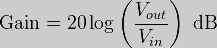
According to the specification of WAT-120N+ the manual gain control allows values in the range of 8-38 dB which if the gain is logarithmic will mean the input signal will be amplified between 2.5 and 79 times(?). For our study the exact figure is of a less significance and it is more important that the gain is linear i.e. the output value will be the input value multiplied by a number. If we go back to the Gaussian PSF this will mean that applying gain is effectively amplifying the amplitude of the Gaussian and doing this for all stars in the field and with the same value. After integrating and substituting the value in the stellar magnitude equation this will mean that the gain will come up as a constant added to each magnitude. Because of this the gain does not affect the linearity of the magnitude differences derived by measured intensity ratios i.e. all stars will appear brighter with the same number of stellar magnitudes.
Anti-blooming Effects
Anti-blooiming is a technology used in CCD cameras to prevent saturation of very bright objects. The following is an extract from the AAVSO, 2004 [10] CCD observing manual about standard CCD cameras: The "anti-blooming gate" is a feature on some CCDs to prevent electrons from leaking
from one pixel to another. This happens when a star is bright enough to "saturate" the
pixels on the camera, filling up the wells. What is left over "leaks" onto adjacent pixels.
This causes spikes and other artifacts in the image. ABG mitigates this effect by putting
"gates" between the pixels. However, this can destroy linearity of the chip and your
photometric accuracy will go along with it.
The "anti-blooming gate" is a feature on some CCDs to prevent electrons from leaking
from one pixel to another. This happens when a star is bright enough to "saturate" the
pixels on the camera, filling up the wells. What is left over "leaks" onto adjacent pixels.
This causes spikes and other artifacts in the image. ABG mitigates this effect by putting
"gates" between the pixels. However, this can destroy linearity of the chip and your
photometric accuracy will go along with it.It is highly recommended that you purchase a camera without ABG. Many manufacturers sell cameras with ABG removed or else have documentation on how you can remove it yourself (if you are brave and mechanically inclined). Another advantage to not having ABG is your CCD sensitivity will be greater.
However, if you end up with ABG in your camera all is not lost. In that case, a good rule of thumb is to limit your pixel saturation to 50% of your well depth. Most cameras with ABG stay linear in this range. For example, most 16 bit cameras stay linear to 32,000 units or less per pixel. Your software will be able to tell you the saturation of a pixel and your CCD documentation will tell you the well depth of your pixels.
Each of the two Sony CCD chips used in WAT-120N+ and PC164C-EX2 are advertised as having 'Excellent antiblooming characteristics' ([11], [12]). I contacted both Watec and Sony asking for more details and what exactly 'excellent antoblooming characteristics' mean. From Watec I got a reply that "SONY have never provided the data of quantum efficiency of CCD sensors to us" and the guy from Sony never called me back.
On the left is an image from the book "A practical guide to CCD astronomy" from authors Patrick Martínez and Alain Klotz which shows the anti-blooming effects in Texas Instruments TC 241 CCD. From the descriptions we learn that there are two ways of implementing anti-blooming - by an anti-blooming drain and using 'vertical' antiblooming system. Searching more about the differences between the two technologies reveals ([13]) that horizontal antiblooming allows for 50 to 100 times overexposure while vertical antiblooming allow more than 100 times overexposure. Because in scientific astronomy anti-blooming is undesired modern CCD cameras produced purely for scientific astronomy (rather than pretty pictures astronomy for example) either allow the anti-blooming to be switched off or provide linearity to 80% or more. It is however unclear how much and what type of anti-blooming is implemented in the low-light video cameras which are mostly produced for security systems.
Based on the figure of the anti-blooming of TC 241 CCD we could however try to model what the effects of this type (and amount) of anti-blooming would be and then try to measure it.
In almost all of the videos I processed for this article the FWHM of a star was typically about 2.5 pixels. This means 95% of the star intensity is spread across a circle with a diameter of 5 pixels. Considering a Gaussian with FWHM of 2.5 pixels we can compute the relative intensity of all the 25 pixels. We can then model how many of them will be affected by the anti-blooming and compute the change in the measured intensity of the star caused by the anti-blooming. For my model (which data can be downloaded here) I did the following assumptions which are based on the TC241 data above:
- The anti-blooming effect starts at 65% of the normal saturation level (I used 65% instead of the 56% from the diagram above)
- The values in the anti-blooming area are linear and are Iab = 0.4 * I
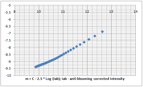
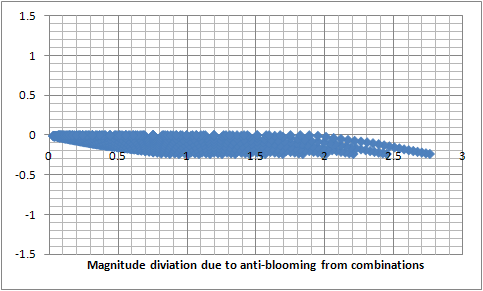
I then modeled the stars as 5x5 pixel features with a Gaussian distribution of 2.5 FWHM (which corresponds to Sigma = 1.6) and computed their intensity as the sum of the 25 pixels. I then built a dataset with a range of amplitudes for the Gaussian and corrected the values for the pixels above 65% (166/255) before adding them up to compute the anti-blooming corrected intensity for each of the modeled stars. Then deriving the magnitudes from the uncorrected intensities and using magnitudes in the range of 10 - 13 mag I plotted the magnitude deviation from magnitude difference curve (the blue plot to the very right), magnitude deviation from magnitude (the purple plot in the middle) and the magnituide deviation from intensity (the plot on the left).
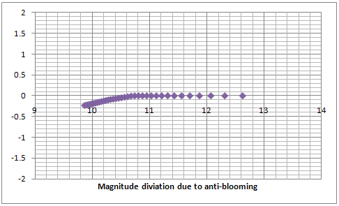
The model shows that the deviation from the true magnitude due to the anti-blooming is up to 0.25 stellar magnitudes and affects stars in the region between 75% and 100% of the full range of detected magnitudes in the modeled video frame. This is certainly something difficult to be measured with a great certainty considering the large random error of the measurements. However that figure is definitely something possible as the existing data cannot reject it either. Further more during all the tests I was sometimes getting plots which deviation could not be explained and have the characteristics of a deviation due to anti-blooming effects.
The three plots below show such a suspicious trend.
Hristo Pavlov, 24 October 2009