Video Photometry with Tangra - Algorithms and Acuracy
Random Error and Photometry Reduction Algorithms
The observed random error from the gamma correction tests cannot be only explained by the uncertainties from the UCAC2 star magnitudes and the spectral sensitivity (which is very close to the UCAC2 band). As mentioned earlier those errors would be expected to be around 0.1 - 0.2 magnitudes for relative measurements such as those in the gamma test. The observed random error was however bigger than that.Tangra is a new software so a valid question will be to estimate the errors introduced by the software reduction itself. It is important to test whether the results in this article that are based on data reduced with Tangra will match closely the results that could have been achieved by using LiMovie. Because LiMovie is currently the only public software used for light curve and photometric measurements of videos and it has been historically used for this purpose I feel that it is important to test and compare the random errors of LiMovie and Tangra. Before doing the comparison let's quickly discuss the photometric algorithms used in Tangra.
Aperture Photometry in Tangra
Tangra uses a standard aperture photometry where it computes the sum of the intensities of all pixels in a measuring aperture. It then computes the average background per pixel from an annulus placed around the measuring aperture and subtracts the background from each of the pixels in the measuring aperture. Differently to LiMovie however, Tangra places the measuring aperture and the background annulus automatically and it possibly uses a different algorithm to compute the background sky level from the background annulus.In Tangra a 3-dimensional (bivariate) Gaussian is fitted for each of the stars in the frame. This allows the determination of the size and location of the star spot with sub-pixel precision. It has been demonstrated (Mighell, K., 1999 [4]) that an aperture with a radius of ~ 1 FWHM gives very good results for aperture photometry. In all tests in this article I used a measuring aperture of exactly 1 FWHM where the full width at half maximum is derived from the fitted Gaussian point spread function (PSF) with a sub-pixel accuracy. The measuring aperture is placed at the center of the star again derived from the coordinates of the center of the fitted PSF and this is done with a sub-pixel accuracy as well. Being able to achieve sub-pixel centering means we should do sub-pixel measurements.
There are a number of algorithms used for sub-pixel photometrtic measurements (for a discussion on the topic see Mighell, K., 1999 [4]). Tangra uses a modified version of one such algorithm, namely the QUADPX algorithm from the CCDCAP package (Mighell, K., 1998 [9]). The idea behind the algorithm is to divide each pixel into NxN subpixels and assign to each of them an intensity of 1/N*N of the intensity of the original pixel. Then rescale the center of the aperture and the aperture radius by a factor of N and compute the sum of the intensities of the sub-pixels inside the scaled aperture.
When computing the sum of the sub-pixels either the whole sub-pixel is included or is excluded from the sum. The test is whether the distance between the center of the aperture and the center of the sub-pixel is greater or smaller than the size of the aperture. If the distance is smaller or equal then the sub-pixel is included in the sum for the signal measurement.
Tangra divides each pixel into a matrix of 5x5 sub-pixels which is a total of 25 sub-pixels. It also computes and stores the number of pixels used in the measuring aperture as a floating point value as: Num(pixels) = Num(subpixels) / 25. Later this value is used to subtract the background from the measuring aperture.
While most packages for aperture photometry are doing the signal measurement using very similar methods, many of them are using different methods for determining the sky background. Some of the programs offer a number of different ways of measuring the sky background. For example, some of the methods deal with diffuse background from nebulas and galaxies by fitting a first or second order bivariate function. While this could be beneficial for example for Lunar occultations and grazes, where the glare from the moon will create a gradient background, handling this type of background is not currently addressed in Tangra.
To measure the background Tangra places an annulus with inner radius of 2.6 FWHM and an outer radius with value that will guarantee at least 350 pixels in the annulus. For example, with FWHM = 3.5 pixels, the inner radius of the annulus will be 9.1 pixels and the outer radius will be: SQRT(350 / PI + 9.1 * 9.1) = 14 pixels. The annulus is centered at the center of the measured star with a precision of 1 pixel. No sub-pixel measurements are used when determining the sky background.
Tangra offers three algorithms to determine the sky background: (1) deriving the background from the PSF fit; (2) computing the background by fitting I = Const using least squares and then excluding all points that are more than 1 sigma away; and (3) determining the background as the mode of the pixel distribution. In all aperture photometry measurements presented in this article I used the third method which is also the method of choice in the DAOPHOT photometry package Stetson. P., 1986 [2].
The mode of the pixel distribution is the brightness value that occurs most frequently in the background annulus. Philosophically this gives a good estimate of what the sky brightness is expected to be. For example this method will be able to successfully exclude stars and on-screen display symbols that may appear in the background annulus. To determine the mode of a population of discrete values, Tangra uses an algorithm initially developed for the "Mountain Software" package at Kitt Peak which is also used by the DAOPHOT package (see Stetson. P., 1989 [3]). Generally Tangra computes the median and mean discrete values of the population of the background pixels and then excludes all values that the more than 6 standard deviations away. It continues to do this iteration until the median and mean stop changing. Then mode of the background is calculated by:
Mode = 3xMedian - 2xMean
Once the mode is calculated it is multiplied by the number of pixels in the signal aperture and is subtracted from the measurement of the signal aperture to compute the final intensity of the star.
Aperture Photometry Results - Comparison between LiMovie and Tangra
To compare the measurements of LiMovie and Tangra and more importantly the random errors, I did a second measurement of my first video used in the gamma correction tests.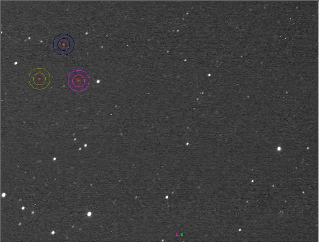 This time I prepared the list of all measured stars and checked the values by eye before generating the star pairs. From all 89 stars I rejected all that had at least one saturated pixel in at least one frame. I then rejected a number of stars with too large errors for the measured intensity as well as rejected 3 stars which measured intensity didn't look right for their catalog magnitude.
I then manually measured in LiMovie each of the remaining 60 good stars measuring 3 stars at a time (and this took a while, but was quicker than I thought it would be). The image on the right shows LiMovie in the process of measuring of one of the groups. I used an aperture of 5 pixels and annulus with inner radius of 12 pixels and outer radius of 21 pixels. I measured the stars in at least 128 frames, then exported the values in CSV, computed the average value and put this value as the LiMovie measurement of the star. The Raw Data in Excel Format is available for download.
Once I measured all 60 stars in LiMovie I did another review of the results and rejected another 2 stars for which the LiMovie measurements were not looking good. The 2 excluded stars were faint (fainter than 12.8 mag).
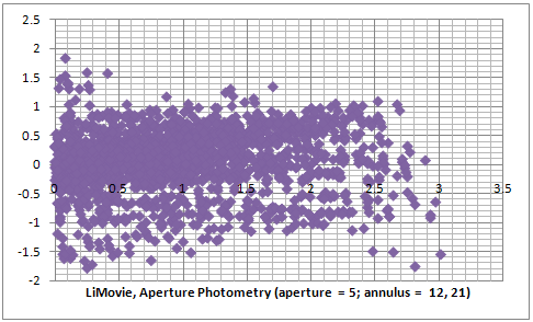
Now having 58 stars with good measurements in both Tangra and LiMovie I grouped them in pairs using all their combinations without repetition but this time made sure that the faint star will be always first (i.e. the higher magnitude will be fist). By doing this I changed the V-shaped curve to a line as m1-m2 will be greater than zero for all pairs. The results are shown below.
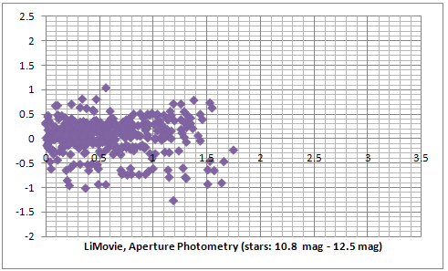
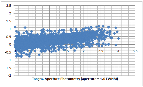
It is evident that the gamma correction effects are also detectable in the LiMovie measurements (in purple) and both LiMovie and Tangra curves have the same inclination. The random error in LiMovie is very close to this in Tangra and is about 0.4 mag for the majority of the stars. One difference is that LiMovie had a greater error for the fainter stars which was also evident from the measured intensities in the raw data spreadsheet. The majority of the scattered pixels on the first purple plot (that have y < -0.5) are actually caused by pairs containing a faint star. The second plot still shows LiMovie data but this time all stars in the region 12.6 - 13.8 mag were excluded. Comparing the second and the third (blue) plot shows that the aperture photometry in LiMovie and Tangra give almost the same results with the same random error for the brighter stars. Comparing the first and the last plot shows that Tangra handles better fainter stars which is most probably either due to the automatically placed aperture with size 1 FWHM, centered with a sub-pixel accuracy at the center of the fitted Gaussian PSF or due to the background calculation algorithm used in Tangra.
Profile-Fitting Photometry in Tangra
A profile-fitting photometry (also known as PSF photometry) is an alternative to the aperture photometry and is largly used in many of the photometry packages. It generally gives more accurate results and allows resolving crowded fields where the stars overlap (for crowded field photometry see Stetson, P.B. 1986, [3]). There are a number of different algorithms for PSF photometry and generally they can be divided into analytical or numerical and differ in the point spread function used and the grouping of stars. The general idea is that if we can fit a PSF function (which is not necessarily a Gaussian) we could integrate it analytically or numerically and derive the intensity of the star. To achieve a better precision in high precision photometry (where errors can be better than 0.01 magnitudes) usually one PSF function is fitted for the central part of the star and another one for the wings as this has been found to represent better the brightness distribution. For a discussion and comparison between PSF and aperture photometry see Fadeyev, V. 2004, [5]. For our purposes in videos, that have lower photometric resolution, we will assume that the PSF is a pure Gaussian.The intensity of a point with coordinates (x, y) of a star with center (x0, y0) will then be:
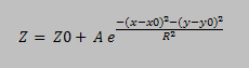
Where A is the height (amplitude) of the PSF and Z0 is the sky background. When measuring the intensity of a star we want to subtract the background Z0. Then the total intensity can be calculated from the integral of the Gaussian. Before doing this we will also apply an encoding gamma correction as a video camera using gamma correction will do. Then integrating the gamma encoded Gaussian we get:

For the duration of the video record we can assume that the sky conditions such as seeing don't change much. This means that all PSFs of the different stars should have the same Sigma. In the equations above instead of Sigma we used R = SQRT(2) * Sigma and this also means that R should also not change from one star to another. If we now use the analytically calculated intensity we can determine the stellar magnitude for each star:
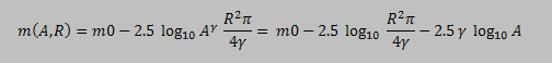
Now, because all stars should have the same R but different amplitude A, then for the stellar magnitudes of the stars in the video we will have:
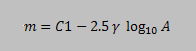
This gives as another way of determining the stellar magnitudes of the stars, this time from the amplitude of the Gaussian. It also gives us a way to determine the encoding gamma of uncorrected for gamma video which we are going to test later on.
Comparison between Results of Photometric Algorithms in Tangra
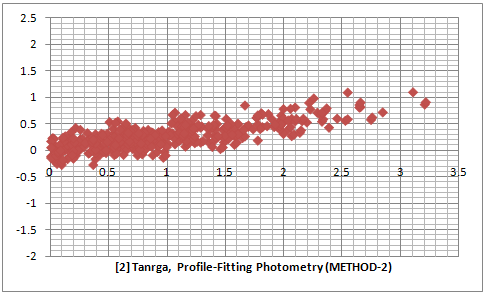
Although the sigma of the stars in a video should be the same, a small variance is observed because the number of pixels per star are usually not large enough for a perfect PSF fit. In order to deal with this some packages (such as DAPHOT Stetson. P., 1986 [2]) for example use the pixels from a number of bright stars shifted and scaled in order to achieve a better PSF fit and determine a better value for Sigma.In Tangra for the tests in this article I used two methods for PSF photometry. The first one (referred to as METHOD-1) simply uses the amplitude A of the individually fitted Gaussians. The second method (referred to as METHOD-2) determines an average value for Sigma from all recognized stars in the first frame of the video. It then uses this as the Sigma of the stars in the video and does a linear least square fit for the amplitude A and the background Z0 for each of the stars, this time fitting a Gaussian with a known Sigma. The amplitude of the new Gaussian is then used to determine the star magnitudes.
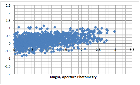
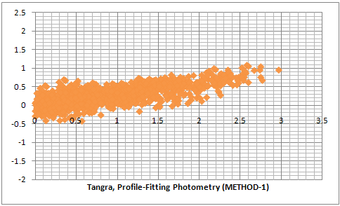
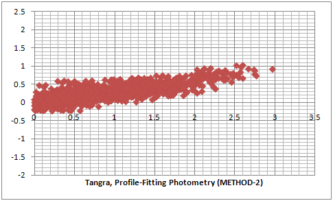
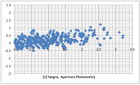
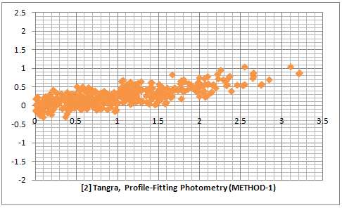
The two series of three plot below are comparison between an Aperture Photometry and PSF Photometry for two different videos recorded with and uncorrected for gamma = 0.45. The raw data for the first three plots can be downloaded here. It is evident that the PSF photometry gives results with a smaller error compared to the aperture photometry. Comparing the PSF photometry methods we see that METHOD-2 gives slightly better results than METHOD-1.
The results from the plots above give an estimate of the relative error when fitting all stars in the field and across all magnitudes (of non saturated stars). In those test the values for the amplitude of the Gaussians were determined after averaging the values from a large number of frames so the random noise in the individual frames has been removed by the averaging process. For reducing video light curves it is also interesting what will be the effect from the different photometry methods on the random noise from one frame to another. In order to test this I measured the same fragment from a video of an occultation of a star by the asteroid (106) Dione. I choose this video because there is a cloud passing through the field of view shortly before the occultation and I wanted to see how the different algorithms will handle this. I measured the video with LiMovie and Tangra.
The plot on the left is measured with LiMovie using a signal aperture of 4 pixels and background annulus of 11 and 19 pixels. The plot in the middle is reduced using aperture photometry in Tangra and the one on the right is done using PSF photometry METHOD-1.
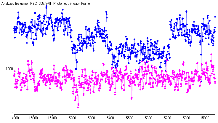
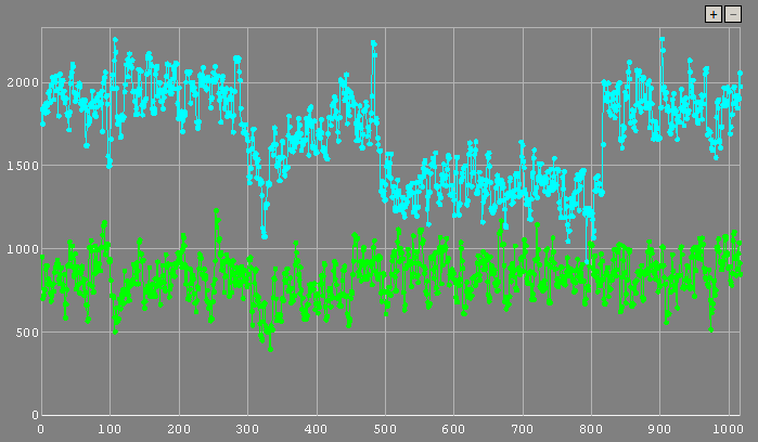
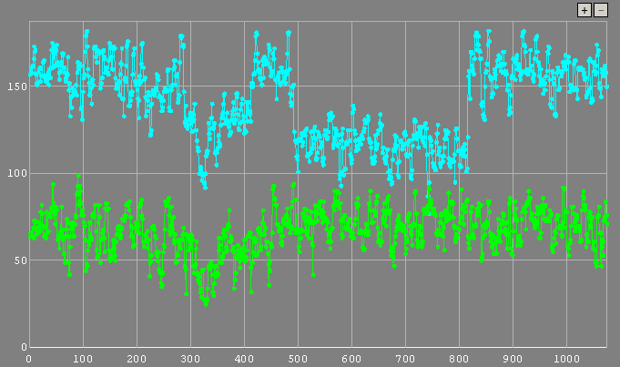
The three plots are very similar but it looks like the PSF photometry plot reveals a finer detail of the passing cloud and the readings during the occultation look slightly more consistent. The LiMovie plot seems to show more noise compared to the other two plots but there is no huge difference in the noise in each frame between the three methods. Knowing the results from the previous test and looking at the three consistent levels of the non occulted star, (1) before the cloud, (2) between the cloud and the occultation and (3) after the occultation it may be suggested that the PSF photometry plot may show a more accurate representations of the real light curve but of course there is no good way to test whether this is true.
From the analytical integration above we got an equation that could allow us to determine the value of gamma. Let's see whether we can do this. The next plots are from a video recorded with gamma = 1.00 (OFF) and processed in three different ways. The first plot is an aperture photometry, the second one is PSF photometry based on the amplitude of the fitted Gaussian and the third one is PSF photometry but this time the fitted Gaussian is numerically integrated in a radius of 1 FWHM. The plots include 24 stars in the range 11.8 - 13.5 magnitudes and the raw data is available here.
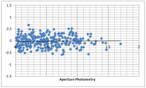
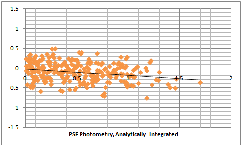
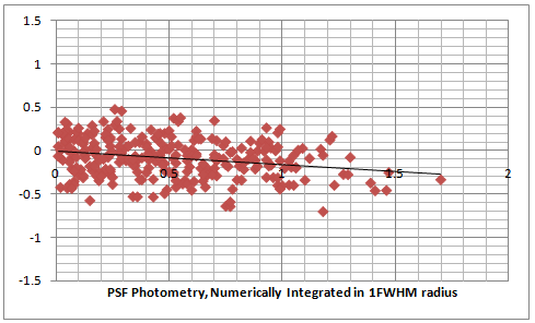
There are a couple of interesting observations. Firstly the aperture photometry of the video recorded with gamma = OFF doesn't have a deviation from the catalog magnitude differences and this is what we would have expected for gamma = 1.00. Then the PSF photometry actually shows a deviation of about 0.1 magnitudes per 1 magnitude difference. This is certainly different from the analytically determined solution as we would have expected that there is no diviation. The last plot which uses numerical integration in an area of 1 FWHM around the center of the star shows the same diviation. Other plots of PSF photometry with videos recorded with gamma = OFF showed the same results. We can therefore say that even that the PSF photometry from a Gaussian PSF gives smaller errors compared to aperture photometry, it does not seem to be linear for gamma of 1.00. Still the deviation is much smaller than the random error.
In all tests until now I was applying filtering to exclude those stars that look bad and don't fit very well. An interesting test will be to this time include all stars that have been detected in say 80% of the frames and we don't reject any of them because of large residuals when trying to fit lineary all magnitudes to the logarithms of the measurements.
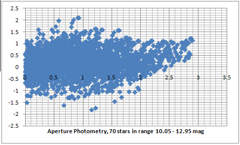
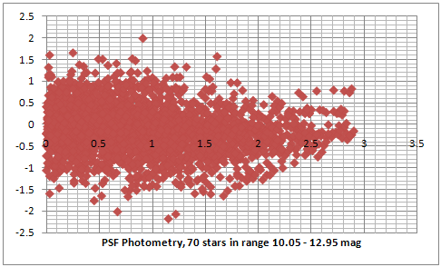
In the next test I use a video recorded with red filter only and with gamma = 1.00 for which the automated processing this time gives 70 good stars, this is non saturated stars that have been detected in most of the frames. For this test only I included 3 stars that have shown saturation correspondingly in 2%, 3% and 6% of the frames. Not including those stars showed neglectable differences in the plots. The raw data can be downloaded here.
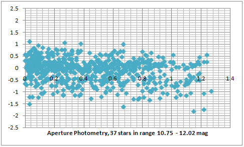
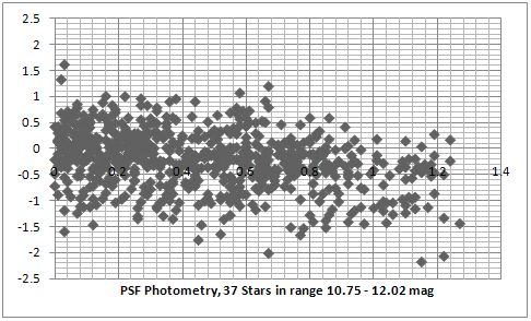
The first two plots (darker blue and red) show the results from aperture and PSF photometry. We can now see that the random error has doubled when using comparison between stars in the full magnitude range of 10.05 to 12.95 magnitude. Also it is evident that the aperture photometry gives a deviation (the right end of the darker blue plot) when comparing stars with larger magnitude differences (between 2 and 3 magnitudes). This means that it either makes the bright stars look brighter or the faint stars look fainter than they are. The PSF photometry still shows a very small deviation of around 0.1 mag per magnitude difference. In the second two plots (lighter blue and dark gray) I removed almost half of the stars equally from the bright and the faint end. This also made the full range of magnitude difference 2 times smaller (from 3 magnitudes to 1.4 magnitudes). Only plotting stars in the middle range should remove all effects of near saturation non linearity (such as antiblooming) and too large errors when measuring very faint stars. The plots don't look very different and the error is still close to 1 magnitude.
A serious issue about explaining the results from the random error is the very small standard deviation of the frame measurements. Most of the stars in the plot above have been identified and measured in more than 200 frames. The average standard deviation for all of the aperture photometry measurements is only about 5 points, which is between 0.3% for the bright stars and goes up to about 2.5% for the very faint stars which corresponds to an error between 0.003 stellar magnitudes for the bright stars to 0.02 stellar magnitudes for the faint stars.
Some of the explanations could be that (1) the magnitudes in the UCAC2 catalog are actually with a bigger error, (2) that the spectral sensitivity of the video camera actually has a much bigger effect or (3) that some of those stars are variables. The first two of these possible explanations will be tested next.